


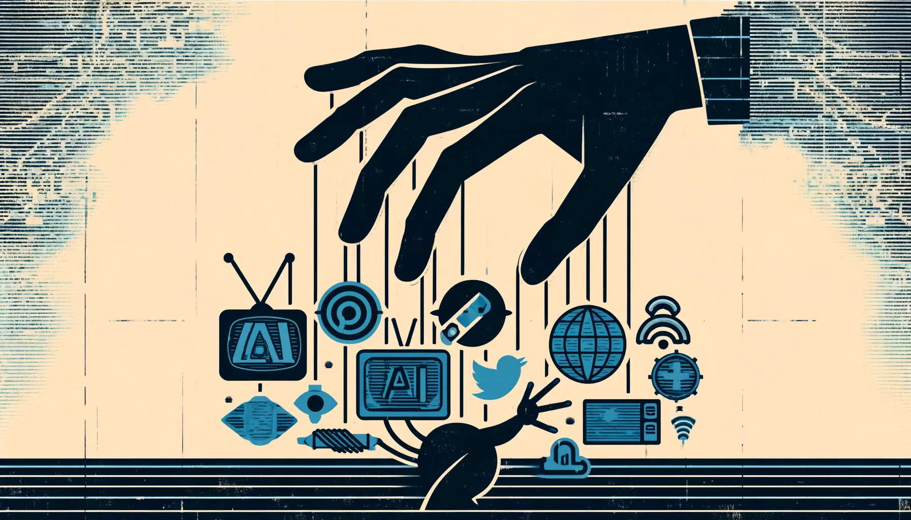
AI Generated Images
image Generated Ai The craze is so much that it took just 1.5 years for AI-generated images to reach the same number as those created by conventional photography!

As goes with everything that appears bright, AI-generated images too come with a huge inherent risk. Look at this photo of the pope wearing a puffer jacket in a fashion show. Quite funny right? The same could be said for this photo of Elon in his monk mode. But for the one shown next, it’s not funny anymore.
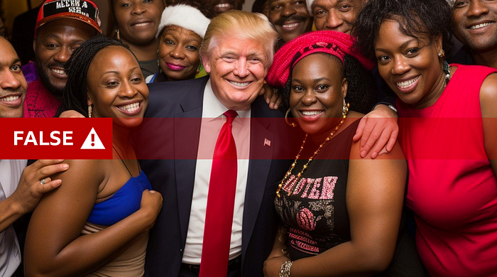
Such AI-generated photos can be used for political propaganda and spreading mass misinformation, and this demonstrates how real harm can be caused by generative AI. Such images need a strong watermark to identify them as AI-generated and to find the person/organisation who created them. Luckily, researchers from Meta have found a way to make this possible. Their latest method, called Stable Signature, allows the addition of an invisible tamper-proof watermark to images generated by open-source AI models specifically Latent Diffusion Models/ Stable Diffusion.
Let’s learn about what these are, first.
An Overview Of Generative AI
Let’s start with the definition of Generative AI. These are AI models that generate different types of data (images, text, video, audio etc.) by learning the patterns and structure of their input training data.The popular types of Generative AI models are described below —
Generative Adversarial Networks (GANs)
These models consist of two neural networks namely, a Generator and a Discriminator that compete against each other during their training process.
Variational Autoencoders (VAEs)
These models are trained by encoding their training data into a latent/ hidden space and then decoding it back to reconstruct the original input.
Autoregressive Models
These models learn to predict future data points in a sequence by learning the patterns in the earlier data points. ChatGPT is a famous example of such a model.
Energy-Based Models (EBMs)
These models are trained to assign an energy score to each data state in the training data and generate new data by finding configurations that minimize the overall energy score.
Diffusion Models
These models are trained by first adding noise to the input data and then reversing this process to reconstruct the original input data over a series of steps.
Let’s learn about diffusion models in a bit more detail.
How Do Diffusion Models Work
Diffusion models are inspired by the physical process of Diffusion where particles present in areas of their higher concentration move to areas of their lower concentration, eventually dispersing evenly in an equilibrium state.
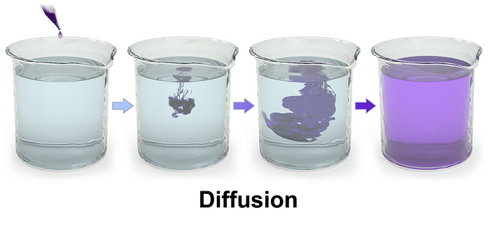
A Diffusion model is trained in a similar way using two diffusion processes.
- Forward Diffusion: The model starts with input data (let’s say an image) and incrementally adds Gaussian noise to it till the data becomes completely random. This process is controlled using a pre-determined noise schedule.
- Reverse Diffusion: In this phase, the model, using a neural network, learns to reverse this noise addition process.
This neural network essentially predicts the added noise at each time step during the forward diffusion process.
The training objective of the overall model is to minimize the difference between the predicted and the actual noise added at each time step.
Once trained, the process of generating new data involves beginning with random noise and iteratively denoising it to create high-quality meaningful samples.

Traditional diffusion models operate directly on the pixel space when generating new images, and hence require a huge number of diffusion steps to generate high-quality results.
This process often consumes hundreds of GPU days and thus is both computationally and financially expensive.
This issue was solved by a group of researchers who proposed generative models called Latent Diffusion Models.
Let’s talk about these next.
What Are Latent Diffusion Models?
Latent Diffusion Models are diffusion models that instead of operating in the pixel space of images, operate on the latent space of powerful pre-trained autoencoders.
This makes their training computationally efficient and less time-consuming.
Here is how they are trained.
- Encoding: A neural network called Encoder takes an image and converts its pixels into their latent representation (with lower dimensionality as compared to its original form)
- Forward Diffusion: Gaussian noise is added to this latent representation till the data becomes completely random.
- Reverse Diffusion: This involves training a neural network to denoise the data step by step to recover the original latent representation.
- Decoding: A neural network called Decoder transforms the latent representation back to its original high-dimensional image form.
The overall training objective is to minimise the difference between the predicted noise and the actual noise added at each step during the forward diffusion process.
To generate new images, the trained model starts with noise and iteratively denoises it to reconstruct the desired outputs.
Note that the Forward and Reverse Diffusion steps are similar to the traditional Diffusion model training process but they occur in the latent space rather than the original pixel space of images.

What Is Stable Diffusion?
An important text-to-image model called Stable Diffusion was born out of Latent Diffusion Models in 2022.
The model essentially conditions the outputs of a latent diffusion model using a text prompt.
It uses CLIP (Contrastive Language–Image Pre-training) embeddings that capture semantic information from images and texts.
These embeddings guide the Reverse Diffusion step and help generate images as per the given text prompt.

Now that we know how Stable Diffusion works, let’s move forward to learn how researchers at Meta can introduce a watermark into the images generated by it.
What Is Stable Signature?
Stable Signature is a method of integrating a binary signature/ watermark into images generated by Latent Diffusion Models (LDMs) like Stable Diffusion.
This is done in a way such that these images can later be detected to be AI-generated and can be identified based on who generated them.
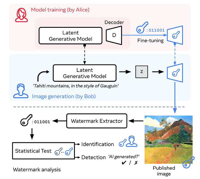
This is how Stable Signature works.
Let’s say Alice trains an LDM and shares it with Bob.
She fine-tunes the latent decoder of this model to embed a binary signature (to identify the model version/ user details etc.) into all its generated images.
When Bob uses this model to generate an image, a watermark extractor can be used to extract the signature from it.
A statistical test can then confirm that the image was produced by the AI model trained by Alice intended to be used by Bob.
Stable Signature works so well because it merges the binary signature/ watermark into the generation process rather than changing the architecture of an LDM (or changing the decoder).
Hence, it can be used with a wide variety of LDMs without altering the quality of the image produced by them.
The method is quite robust and surprisingly works even when —
- the original images are cropped to 10% of their original size
- their brightness is increased twice
- combined changes (cropping to 50%, adjusting brightness by a factor of 1.5 and JPEG 80 compression) are applied
Notably, the method also has an extremely low false positive rate of below 10^(-6).
In other words, in every one million negative (or non-AI-generated) images, the model wrongly flags only one image as positive (or AI-generated when it is not).
A Deep Dive Into Stable Signature
The method involves two phases —
1. Pre-training The Watermark Extractor
This phase is inspired by HiDDeN, a deep watermarking method.
A Watermark Encoder (WE) is given the original image and a k-bit binary message (signature)(m) as its input. The output of this encoder is the watermarked image.
During each optimization step, a transformation (T) is applied to the watermarked image. This is to simulate real-world modifications (cropping/ compression) to the image.
Next, a Watermark Extractor (W) processes this transformed image and a ‘soft’ message is extracted from it.
The actual message is determined by the signs of the components of this ‘soft’ message.
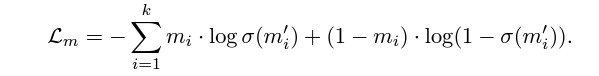
The loss function (Message loss orL(m)) used during this training is the Binary Cross Entropy (BCE) between the original message and the sigmoid transformation of the extracted ‘soft’ message.
After the training process, the Watermark Encoder is discarded since it is no longer needed, and the Watermark Extracter is kept.
2. Fine-Tuning The Generative Model (LDM)
In this phase, the Decoder (D) of the targetted LDM is fine-tuned so that it integrates the embeddings of a selected message (m) in all its generated images so that this can be later extracted by the Watermark Extractor (W).
This modifies the Decoder (D) and this modified Decoder is described as D(m) in the research paper.
Two loss functions are used in combination in this phase:
- Message loss (
L(m)): This is the Binary Cross Entropy loss between the signature extracted from an image (m’) by the Watermark extractor (W) and the original binary message (m).
This loss makes sure that the extracted message (m’) is correctly embedded into the model generations. - Perceptual Loss (
L(i)): The Watson-VGG perceptual loss is used here and this compares the visual quality of the generated watermarked image byD(m)to the image produced by the original decoder (D).
This loss ensures that the quality of the images does not change when they are watermarked.
The combined loss (L) is minimized during training using the AdamW optimizer.
The hyperparameter λ(i) ensures the balance between both the losses.

The overall process is shown below.

Statistical Test Used To Detect The Watermark
To compare the original signature (m) and the extracted signature (m’), the Hamming distance between these is calculated.
This is calculated by counting the number of bit positions in which the two k-bit binary signatures (m and m’) differ.
A decision threshold is pre-decided to determine how close m’ must be to m to consider the image to have been generated by the model.
This threshold is set so that the false positive rate of the model is kept low