A Beginner to Advanced Guide.

The Mathematics behind Mean/Averages. A Beginner to Advanced Guide.

If you’ve ever heard of the term “the average man”, you probably (at least once) have come across the history of the term “mean”. The average man means what it says. It signifies taking the average on every man/woman to produce an “average man”. This was developed by The Belgian statistician, Quetelet. He claimed that if we imagined 1000 flawed sculptures of a statue of a gladiator, on average, they would result in the original. (Mostly because the average cancels out errors — More explanation Later). But then, Quetelet continued, if we measured a thousand real soldiers and averaged their body measurements,

we could get the ideal, perfect soldier. What he forgot was that not all variation is error. A 6’4-foot soldier might benefit from having a superior reach than the “average” soldier. Mean has been used since the Greeks for tackling day-to-day challenges. The arithmetic mean was not the only mean value known to them. In Pythagoras’ time, around 500 BC, three mean values were known. Namely: harmonic, geometric, and arithmetic mean. Most people (including Data Scientists) are only familiar with arithmetic mean (typical average) and hence are unable to quickly solve problems requiring other types of mean. Although you might hardly need some of these mean values, the time you do, they come in very handy. Some job interviewers are also fond of asking trick questions to test your intuition and skills on various types of mean.

This post will discuss each type of mean along with their history, derivations, past vs current formula, Use cases, and disadvantages. This article is not going to be your typical tutorial. More than anything, the article’s purpose is to hone your intuition.

So Buckle up!

If you got here, I advise you to bookmark/save this post for later. I would constantly be updating it with new and mind-blowing information.

Arithmetic Mean

The sum of all observations/number of observations

The arithmetic mean is simply finding the average or center of a given set of values or observations. It takes into account the weight or size of each value respective to others when determining an average.

History

The arithmetic mean was discovered by a Greek astronomer called Hipparchus. It was used to reduce the sampling error in his astronomical observations when determining the position of the sun, moon, and planets.

He found that 0.25% of the time, the predictions he got from his calculations, when taken under similar circumstances (eg In the morning) were inaccurate. But by taking the mean over a period of time, the errors would cancel out or eventually become so minor to the point of obscurity. Aristotle had a famous philosophical quote highlighting the definition of mean and when it is not to be considered…

“By the mean of a thing I denote a point equally distant from either extreme, which is one and the same for everybody; by the mean relative to us, that amount which is neither too much nor too little, and this is not one and the same for everybody. For example, let 10 be many and 2 few; then one takes the mean with respect to the thing. if one takes 6; since 10–6 = 6–2, and this is the mean according to arithmetical proportion [progression]. But we cannot arrive by this method at the mean relative to us. Suppose that 10 lb. of food is a large ration for anybody and 2 lb. a small one: it does not follow that a trainer will prescribe 6 lb., for perhaps even this will be a large portion, or a small one, for the particular athlete who is to receive it; it is a small portion for Milo, but a large one for a man just beginning to go in for athletics.”

To drive your understanding of the quote, when Quetelet, The Belgian statistician, came up with the theory of the “average man”, the sculptor Abram Belskie and obstetrician Robert Dickinson, decided to turn his metaphor into reality. They carved statues (“Normman” and “Norma”) based on the measurement of 15,000 young American men & women respectively.

The Americans Loved Norma.

Norma’s butt is 29 inches across, from hip bone to hip bone. It’s round and pert and, because it’s made of stone, alarmingly smooth. It is substantial, a handful, but no one would call it big. If it were made of flesh, it would fill out a swimsuit nicely, but I doubt it would elicit a long second look. Norma has the Goldilocks butt, the Goldilocks body. Everything about her, at least according to the people who designed her, is “just right.” — TIME

This gained a lot of press. Most women began comparing their bodies to Norma. The statue became a sort of ideal even though it was just made to be average. A competition of 3,863 women was sponsored by the Cleveland Health Museum to find an actual woman who matched her dimensions, but only a minute of people came close. There was no exact match.

It became obvious that being average was just as rare as being perfect. This is an example of “mean relative to us” as suggested by Aristotle. It’s like taking an average of the hair colors of interracial students in a class. You are almost guaranteed not to find anyone with the “average hair color”. Therefore it can’t be the average.

Derivation

By the mean of a thing I denote a point equally distant from either extreme

y₁ = highest_extreme_point
y₂ = lowest_extreme_point
y = average / mean

y¹_deviation = y¹ — y (positive deviation)
y²_deviation = y — y² (negative deviation)

From the equation above, we can derive the formula for arithmetic mean:

The goal of the mean is to calculate a central tendency given a set of numbers or variables. This simply means that the sum of positive deviations is equal to the sum of negative deviations. Positive deviation only considers the data points or numbers greater than or equal to the mean. Negative deviation only considers the data points or numbers less than the mean. For instance, if we have a data set of {1,2,3,4,5}. To get the positive and negative deviations, we would need to first find the mean value.

the sum of positive deviations is equal to the sum of negative deviations:

However, this assumes that all variables or numbers are of almost equal accuracy, length, or value in the dataset.

If we somehow introduce a number such as 1000, we would get a completely biased mean value i.e. our mean value would tend more towards 1000. This is mainly due to the arithmetic mean’s additive nature.

A more robust method of dealing with such is to find the median or geometric mean.

Imagine having 3 random car engineers and Elon Musk in the same room. Who’s opinion do you think would influence the group’s thinking (and hence results) more? (10 + 20 + 30 + 1000) / 4

But this influence lessens when the sample size is bigger. The bigger the sample size of the dataset, the less an outlier has the potential to affect the mean.

Elon Musk vs 10000 car engineers, for example, should be a fair fight.

Another example… Suppose we have a dataset of 100 exam scores where all of the students scored at least a 90 or higher except for one student who scored a zero:

[0, 90, 90, 92, 94, 95, 95, 96, 97, 99, 94, 90, 90, 92, 94, 95, 95, 96, 97, 99, 93, 90, 90, 92, 94, 95, 95, 96, 97, 99, 93, 90, 90, 92, 94, 95, 95, 96, 97, 99, 93, 90, 90, 92, 94, 95, 95, 96, 97, 99, 93, 90, 90, 92, 94, 95, 95, 96, 97, 99, 93, 90, 90, 92, 94, 95, 95, 96, 97, 99, 93, 90, 90, 92, 94, 95, 95, 96, 97, 99, 93, 90, 90, 92, 94, 95, 95, 96, 97, 99, 93, 90, 90, 92, 94, 95, 95, 96, 97, 99]

The mean turns out to be 93.18. If we removed the “0” from the dataset, the mean would be 94.12. This is a relatively small difference. This shows that even an extreme outlier only has a small effect if the dataset is large enough.

Typically, we mainly use arithmetic mean for arithmetic sequences. These are sequences where each new term is obtained by adding a constant number to the preceding term. This constant number is referred to as the common difference. eg. {10, 20, 30, 40, 50}

When should I use Arithmetic mean?

1. Your variables are of equal value to your intent
2. Most of your variables are of close range and have a linear pattern of increase/decrease [arithmetic sequence].
3. Your data set should be balanced i.e. Most of your variables must be spread out and not on either extreme. (eg. highest or lowest, closer to 1 or 10, very poor or very rich)

Geometric Mean

Using our previous instance of Elon Musk and 3 random engineers, what if the value of the first engineer’s opinion is multiplied by the value of the next engineer’s opinion, and so on? We’ll find that very quickly, there won’t be much space for Elon to have an influential opinion.

The geometric mean is less sensitive to outliers due to its multiplicative nature i.e. 2 + 100 = 102 but 2 * 100 = 200; the lack of value in 2 has been compensated by 100.

The geometric mean is calculated by multiplying all values in the data set and then getting the nth root — n is the size of our data set.

Why the size of our data set? Because we are trying to find a value that when it multiplies itself a certain number of times (n in this case), can give us our total value.

5 * 5 = 25. Square root of 25 = 5
5 * 5 * 5 = 125. Cube root of 125 = 5

nth root value is calculated in order to revert to the default scale/range of our values/variables. e.g. from the example above, the square root of 200 is 14.1. The value is now a lot closer to 2 than it is to 200.

The geometric mean is used when the values of the data distribution change multiplicatively or divisionally (eg. 1, 3, 9, 27, 81…). — The value/distance between two numbers is the same both multiplicatively or divisionally, e.g3 * [9] = 27, 27/3 = [9].

Typically, we mainly use geometric mean for geometric sequences/progressions. These are sequences where each new term is obtained by adding a constant ratio to the preceding term. This constant number is referred to as the common ratio. eg. {2, 4, 8, 16, 32}

This makes it ideal for averaging data that has some multiplicative relationship, such as ratios, compound interest, etc.

If we had Jeff Bezos, with a starting salary of $100,000, had an increase of 3%, 6%, 12%, 24%, 32% for 5 years. What was his average annual interest rate?

Naively, we might want to use arithmetic mean: 1.03 + 1.06 + 1.12 + 1.24 + 1.32 = 5.77

We added 1 because the formula of compound interest is —
Principal * [(1 + interest rate)ⁿ— 1]

n — number of compounding periods

5.77 / 5 = 1.154%, therefore using the compound interest (CI) formula:

Total interest earned = $100,000 * ((1.154)⁵ — 1) = $104,658.15
Interest + principal = $104,658.15 + 100,000 = $204,658.15
Final total = $204,658.15

But let’s do it ourselves

$100,000 * 1.03 = $103,000 or (100,000 + ($100,000 * 0.03)) = $103,000
$103,000 * 1.06 = $109,180
$109,180 * 1.12 = $122,981.6
$122,981.6 * 1.24 = $151,629.184
$151,629.184 * 1.32 = $200,150.5
Total earned = $200,150.5

By using the arithmetic mean, we were off by $4,507.

Let’s use geometric mean

1.03 * 1.06 * 1.12 * 1.24 * 1.32 = 2.001505
5th root of 2.001505 = 1.149

CI = 100,000 * (2.001505–1) = $100,000 * 1.001505 = $100,150.5
Total = 100,000 + 100,150.5 = $200,150.5

We didn’t use the 5th root (1.149) because we would just end up squaring it back up by 5 and getting the same result.

As we can see, geometric mean was a more accurate measure of central tendency than arithmetic mean in this scenario.

In what situations should you use Geometric Mean?

1. The variables/values have some multiplicative or exponential relationship between them.
2. There are outliers in the data set.
3. The variables are of different scales or units.

Harmonic Mean

I do not have a very broad understanding of harmonic mean so I would use the little I have to explain. When I do, I will update this post.

History

In the time of Pythagoras, there were only three means (Bakker 2003; Brown 1975; Huffman 2005), the arithmetic, the geometric, and third that was called subcontrary, but the “name of which was changed to harmonic by Archytas of Tarentum and Hippasus and their followers, because it manifestly embraced the ratios of what is harmonic and melodic” (Huffman 2005, p. 164).

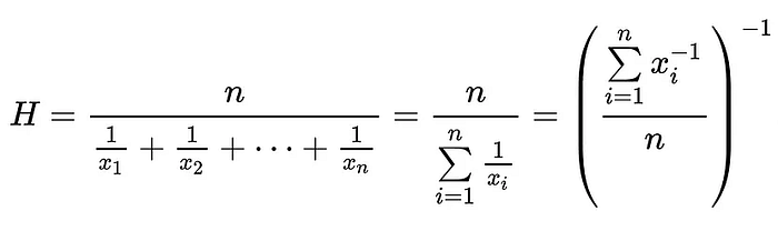
The harmonic mean is a measure of location used mainly in particular circumstances — when the data consists of a set of rates, such as prices ($/kilo), speeds (mph), or productivity (output/manhour). lt is defined as the reciprocal of the arithmetic mean of the reciprocals of the values.

It appears from an examination of the treatment of the harmonic mean (the reciprocal of the arithmetic mean of the reciprocals of the items being averaged) in a number of the popular textbooks on statistical methods, that there is a good deal of doubt and misapprehension in the minds of even our experts as to its true nature and usefulness. The current confusion was vividly brought home to the writer a few years ago the first time he tried to explain its use to a class of college juniors. Having been taught that the harmonic mean should be employed in averaging time rates, he used the example of the average rate at which three men load dirt into a wagon, one loading two, another three, and another four wagons per hour. Seeking to show that the arithmetic mean of three loads per hour was incorrect, he found, in front of the class, that it was perfectly correct if it be agreed that the men all work the same length of time. Several texts consulted at that time failed to elucidate the problem; some have no mention of the harmonic mean, while others merely give its definition with no consideration of its nature or use. Some texts give illustrations which are valid, but incomplete for a full understanding of the problem; a few give misleading and even impossible illustrations.

Seems I am not alone. If you really grasp this concept, please state in the comments for $5.

[ +- ] — Arithmetic mean
[ *÷ ] — Geometric mean
? — Harmonic mean

Harmonic mean utilizes reciprocals i.e. the inverse of a number(n => 1/ n ).

A good frame of thinking for reciprocals is what is a number that multiples the number in mind to produce 1.

If you have any value in your dataset that is 0, the harmonic mean would always return undefined because no reciprocal can multiply 0 to give 1.

The reciprocal of 3 is 1/3.
3 * 1/3 = 1

The harmonic mean is the reciprocal of the arithmetic mean(AM) of the reciprocal of the dataset.

Harmonic mean — 1/R[AM]
R[AM] — reciprocal of the dataset/size of the dataset

1. Take the reciprocal of all values in the dataset
2. Find the arithmetic mean of those reciprocals — R[AM]
3. Take the reciprocal of that number — 1/R[AM]

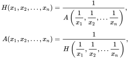
The harmonic mean helps us find multiplicative or divisory relationships between fractions without worrying about a common denominator.

It’s often used for rates and ratios.

One cliche example is traveling over physical space at different rates, i.e. speeds.

For example,

if a vehicle travels a certain distance of 10km outbound at a speed of 60 km/h and returns the same distance at a speed of 20 km/h, what was the vehicle’s average speed?

Pattern recognition heuristics would tell you to simply take the arithmetic mean and voila, you have 40km/h as the mean.

But this is wrong because the vehicle traveled at different speeds over the same distance. So the time taken to cover each distance is smaller at 60km/h and longer at 20km/h.

So your average rate of travel across your entire trip’s duration is not the middle point between 60 mph & 20 mph, it should be closer to 20 mph because you spent longer traveling at that speed.

Using Arithmetic Mean [AM]
To solve this using arithmetic mean, we have to determine the amount of time spent traveling at each distance.

Time taken = distance / speed = 10 / 60 = 0.167 hour
Convert to mins = 0.167 * 60 = 10 minutes
Outbound time taken= 10 minutes

Time taken = distance / speed = 10 / 20 = 0.5 hour
Convert to mins = 0.5 * 60 = 30 minutes
Inbound time taken = 30 minutes

Total time taken = 30 + 10 = 40 minutes

% of Outbound time = 10/40 = 0.25 * 100 = 25%
% of Inbound time = 30/40 = 0.75 * 100 = 75%

Weighted AM = (60 * 0.25) + (20 * 0.75) = 15 + 15 = 30
Average speed = 30km/h

As you can see the average speed is just about 10km/h lower than our previous value of 40km/h. Let’s verify this using harmonic mean.

Using Harmonic Mean [HM]

AM of Reciprocals = 1/20 + 1/60 = 4/60 = 1/15 ÷ 2 = 1/30
R of [AM] = 1 ÷ 1/30 = 30

Average speed = 30km/h

So there you have it. You can use weighted Arithmetic mean or Harmonic mean but you’ll often find it more convenient to use harmonic mean. It’s less verbose and less prone to error.

It’s like choosing addition when trying to calculate 5 in 100 places (5₁ + 5₂ + 5₃ + 5₄ … 5₁₀₀) rather than multiplication (5 * 100).

Ferger, W. F. (1931). The nature and use of the harmonic mean. Journal of the American Statistical Association, 26(173), 36–40.

Read more