


A beginner to Advanced Guide.
The Mathematics behind linear regression A beginner to Advanced Guide. Linear regression is by far one of the most impactful statistical methods used in the 21st century. From computer science to medicine, to geology, to aeronautics, to behavioral and social science, and many more.
Everyone involved in Machine Learning or Data Science must have a strong understanding of linear regression. It’s almost a default. This article aims to help you do justice to that. But in order to do justice to that we’re going to need to go all the way back to the 1800s and 1900s, to understand the thinking behind the thinking. Get a grasp of how linear regression became what it is today.
We won’t be doing a lot of maths or graphs here. Not yet. This article’s existence is mainly to please your intuition. To see Maths as a means by which humans communicate non-verbally at a global scale. We’ll be using this Python fiddle to implement any graphs or plots.
Get a coffee and let’s dive in!
THE FEAR OF ERRORS

THE FEAR OF ERRORS Before diving in, we need to briefly touch on the concept of errors in statistical theory.
Normally we see errors as a mistake, but in statistics, an error is simply just the difference between an estimated value and the actual true value.
For a more in-depth analysis on errors, read this article.
Wikipedia:
In statistics, “error” refers to the difference between the value that has been computed and the correct value.Oxford:
The quantity by which a result obtained by observation or by approximate calculation differs from an accurate determination
Handling errors has always been a problem. Astronomers since the 18th century had a deep-rooted fear of combining observations. The fear was not based on observations under similar circumstances, as those were easily solved using mean, but by observations made under varying circumstances (non-standardized observations). Combining such observations to get an estimated “truth value” was faced with serious skepticism. How this truth value is determined is left to the observer or analyst.
Theodore M. Porter best describes the problem:
“Astronomers had been debating for several decades the best way to reduce great numbers of observations to a single value or curve, and to estimate the accuracy of this final result based on some hypothesis as to the occurrence of single errors.”
This simply means astronomers had difficulties finding a way to standardize varying ranges of observations (eg 1 and 1000), and even after standardizing it to a single range or value, finding a way to properly determine the accuracy gotten from this range or value.
If you don’t know what standardizing means, it’s simply bringing down values within similar ranges. (eg 1 and 1000 * 1/2000 are close in range)
Taking the mean was not an option because the mean value was too far away from most of the individual observations. Most also feared that the errors within each observation would multiply, not compensate, and move greatly away from the supposed “truth value”. How these observations got contaminated with errors could vary which made the problem more relevant. It could be faulty instruments, human error, wrong calculations, atmospheric conditions, etc.
A rule was needed. One that would account for all observations and their variations.
THE INVENTION OF LEAST SQUARES
A man named Legendre came out with a formula that accounts for all observations and their variations. The method of least squares.
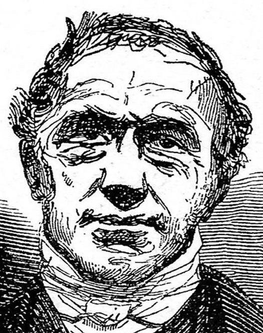
A Brief on Legendre
He was born in Toulouse and the family moved to Paris when he was very young. He came from a wealthy family and he was given a top-quality education in mathematics and physics at the Collège Mazarin in Paris.
The method was highly accepted across all domains. At that time, no statistical method had as much of an impact as this did. It began the acceptance of errors.
Legendre suggested that the sum of the squared deviations around the mean would provide some grand estimate of the error variance on the entire observations.
Remember…
Error is simply just the difference between an estimated value and the actual true value.
We square the deviations because we do not care about direction. We just want a total or an aggregate and hence squares remove any negative operator to make it possible for us to get a grand estimate.
We also square to identify and penalize outliers easily.
For example, if we have a dataset of [10,46,100,2345,832] and we calculate the mean, we get 666.6.
To calculate the sum of the squared deviations, we are going to….
(10–666.6)² +(46–666.6) + (100–666.6)² + (2345–666.6)² + (832–666.6)²
431123.56 + 385144.36 + 321035.56 + 2817026.56 + 27357.16
Total deviation = 3981687
This is an aggregate of how much the dataset deviates from the mean. By quite some margin as we can see (mostly due to the square).
This helps us to know how well our datasets vary from each other. Also, by squaring the difference, we put more weight on outliers which can help us quickly figure out any variables that influence our prediction or model heavily. In our case, 2817026.56 or 2345 is the outlier.
Using graph

Suppose we have all these data points. And we try to plot a best-fit line in order to predict new values…

Our error is the difference between the actual data points (red points) and the line…
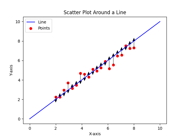
Once we get the difference of each point, we square each difference up and add them to get the sum of squared deviations.
With this aggregate value, we can now try to find the best-fit line (assuming this is not already it), by moving closer to values that drastically influence our aggregate value in order to reduce their deviation.
Our goal with the least square is to minimize the total deviation to as minimal as possible.
This method’s breakthrough was that “errors” could now be combined, but more importantly, minimized through a method that would enhance prediction, not through multiplying error, but reducing the overall quantity of it.
The method gained wide appeal and by the early 19th century, was used regularly in the fields of astronomy, geodesy, and eventually spread to the social sciences, including psychology.
One issue with the sum of squared deviation is that it assumes that your data point follows a normal distribution. eg {20, 18, 23, 22, 15, 24, 20, 29, 16, 19} rather than a skewed distribution eg {25,30,35,40,45,50,55,60,65,70,75,80,85,90,95,100}.
By normal distribution curve, I mean most data points in a set revolve around the mean or some central tendency (eg median) with fewer and fewer data points as they go further and further away from the center. For instance, population, age, weight, height, house prices, etc.

Don’t bother about the mathematical complexities of the image above, just understand how it relates to a normal distribution curve/dataset.
This is particularly one of the reasons why least square is used with regression analysis.
THE FALSE INVENTION OF REGRESSION

A man named Bravais Auguste came first to find the regression line but had no idea he did so. He was a physicist and a professor of astronomy. Most of his works were aimed at crystallography.
He is best known for a paper he wrote in 1846 titled “Analyse mathématique sur les probabilités des erreurs de situation d’un point” translated to “Mathematical analysis on the probability of errors of a point”.
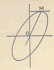
He found what would eventually be coined the “regression line.” He did so by investigating how the various elliptical (oval-shaped circles) areas of the frequency surface vary given various directly observed quantities.
Frequency surface means the frequency or quantity of values in different parts of distribution (both extremes and the middle).
Through this, he found the line of regression, but did not realize it, and thus could not “make the leap”. This was mainly because he didn’t have the goal in mind.
At the time, getting rid of errors from observations was the highest priority and thus, bravais goal was to do just that. His motivation was to show how the errors obtained from observations were independent, not associated.
This blindsided Bravais to the idea of correlation.
He was able to get the line (i.e., “OM”) which is similar to the common regression line. But this is not a result of observing x and y and determining their association, but of the fact that x and y are functions of certain independent and directly observed quantities”
But since he managed to somehow derive the regression line, shouldn’t he be crowned for it? I mean, he was one of the first to study the existence of two or more errors, something that only a few at the time had done before.
Second, he produced the product term for the correlation coefficient and discovered the mathematical equation for what 30 years later was coined the regression line.
Product term for the correlation coefficient
Multiplication of deviations X and deviation of Y divided by the standard deviation
Third, he discussed both of these in terms of the normal surface of correlation and identified the varying shapes of the ellipses that would exist given varying quantities and accompanying errors.
Well, let’s talk about the real father — Galton.
THE INVENTION OF REGRESSION
Galton observed that the mean value of inherited characteristics deviates away from the mean of the mid-parents(average height of both parents) and towards the mean of the population.
Suppose you have tall parents, your height wouldn’t be directly a result of the mean of your parent’s height but more towards the mean height of the entire population.
So if you have extremely tall parents, you are mostly likely to be shorter in stature and if you have extremely short parents, you are most likely to be taller.
The main thesis is that deviations in inherited characteristics could be explained by their regression towards the mean value. Extreme deviations did not produce equally extreme characteristics/deviations but in general, deviations of a lesser degree regressing towards the central tendency, the mean.
A brief on Galton’s motivation…
Galton possessed a penchant for observations, some would even say an “obsession.” In short, Galton measured everything he could, from wind direction to fingerprints, to what would form the empirical roots of his later discoveries — physical attributes such as heights and stature. As Stigler (1986) remarks, Galton was greatly influenced by Quetelet in that he almost “rejoiced” in Quetelet’s concept of a theoretical law of deviation from an average (i.e., “error theory”). Galton even appears to have foreshadowed, using the concept of the error curve, the basis of modern hypothesis-testing, that of determining whether observed values arise from a single population, or from various populations.
He tried to graphically display the distribution of human physical attributes, with the hope of somehow showing that these attributes are inherited. This somehow plagued Galton’s mind which led him to perform an experiment that would calculate a reversion coefficient.
A reversion coefficient is a coefficient of correlation between two variables. This coefficient determines the rate of reversion to the mean and can help with forecasting.
He took a data set of 928 offspring and their parents to produce a Table of Correlation. Such a table plotted the heights of mid-parents against the heights of offspring.

For instance, if a parent was 70 inches in height, and the adult child had a height of 67, a checkmark was placed in the corresponding cell where the two entries formed a 90° angle. (female’s heights were multiplied by 1.08 to normalize the dataset.) These checks were then tallied to produce the numbers in the graph below…
What Galton noticed next was significant to his discovery.
He found that when line segments were drawn that connected each point where the values were the same, the lines formed an ellipse and the center point of these ellipses was the mean of values on the ordinate and abscissa.
He further found that at each point where the ellipse was touched by a horizontal tangent, all points lay in a straight line and each line was inclined to the vertical in the ratio of 2/3.
Those points where the ellipses were touched by a vertical tangent also lay in a straight line but this time inclined to the horizontal in the ratio of 1/3.
By measuring the heights of hundreds of people, he was able to quantify regression to the mean and estimate the size of the effect. Galton wrote that “the average regression of the offspring is a constant fraction of their respective mid-parental deviations”.
This means that the difference between a child and its parents for some characteristic is proportional to its parents’ deviation from typical people in the population.
If its parents are each two inches taller than the averages for men and women, then, on average, the offspring will be shorter than its parents by some factor (which, today, we would call one minus the regression coefficient) times two inches.
For height, Galton estimated this coefficient to be about 2/3: the height of an individual will measure around a midpoint that is two-thirds of the parents’ deviation from the population average.
By doing this, Galton confirmed his invention of statistical regression. Not mathematically, but through empirical data and observation.
One mind-blowing fact was that Galton was not a mathematician. He had no deep roots in maths and even before he concluded his experiment, he sent the data to a mathematician called Dickson to reproduce mathematically what he produced empirically. To his amusement, it was the same result.
Although Auguste Bravais touched statistical regression and correlation, Galton made it law.
Galton also notes that due to the law of regression, he’s very much against the current practice of proportional rescaling because it ignores the effect of regression.
If a thigh bone is 5% greater than the average thigh bone, we should not infer that a man is 5% taller than the average person. Such an inference would ignore the effect of regression and would tend to overestimate by an amount that is greater than even those on the extreme of the distribution curve.
CONCLUSION
Perhaps there is no better example in the history of statistics than the one before us to show that statistical techniques do not simply arise out of mathematical manipulation, but are often spun out by a social-political cause or other equivalent goal.
Hence, in this context, the statistical technique is but a “weapon” in the pocket of artillery of the proponent. Since Bravais had no particular reason for finding the technique of correlation, he did not.
Similary, since Galton’s theory of inheritance relied heavily on him finding a “mechanism” of inheritance, he had all the reason and motivation for discovering the technique of regression and correlation, and so he did.