


How to learn what treatments are best for whom, how we use this at Klaviyo to power a new AI feature, and how we accidentally (re)invented it from first principles.
Part One: How we accidentally (re)invented Uplift Modeling
In March 2022, it had been a year since we released our Klaviyo SMS product. We wanted to guide our customers (email and SMS senders) to use both channels effectively. A few data scientists and myself were gathered to discuss a research proposal RFC, a data science version of Klaviyo’s RFC where a data scientist’s peers review their planned work.
The RFC proposed to run experiments on ways to identify which campaign recipients should receive an SMS and which should receive an email instead. We had 5 rules in contention. For example: sending SMS to customers who had just consented to receive SMS and sending email to everyone else.
Complicating the matter was our suspicion that every profile in general would be more likely to engage if sent SMS. So, we needed to understand not just which channel would be better, but by how much.
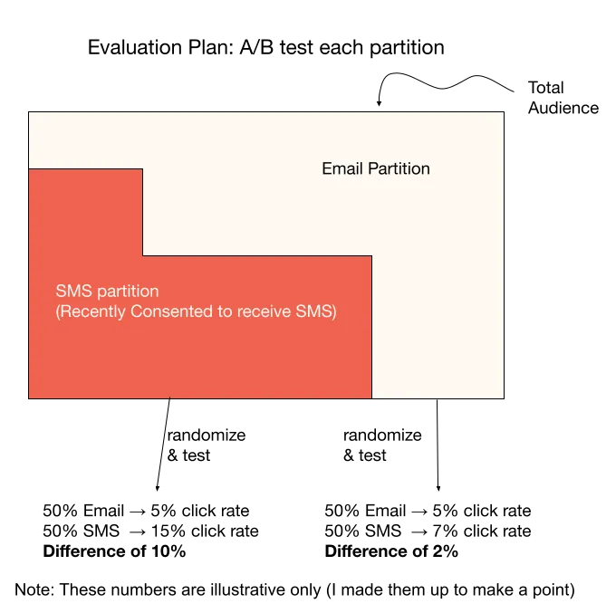
The proposal was to run an A/B test, something we’re used to at Klaviyo. Each strategy produces a partitioning of a campaign’s recipients, where one partition would be the email partition and one would be the SMS partition. We’d send half of the profiles in each partition SMS and half Email. If our partitioning was good, the difference in performance between SMS and Email would be higher for the SMS partition than for the Email partition.
Unfortunately, since there were so many strategies to test, this plan would take a lot of time and effort; we could only test one strategy per experiment. Too many experiments, too much time! How could we possibly test all of these different strategies with limited data? Or have confidence that we did a good job, given there are infinite possibilities?

That’s when we made a key observation: segmenting recipients into groups and then randomizing the treatment (Email or SMS) is mathematically equivalent to randomizing the treatment and then segmenting recipients. In other words, we could save a lot of time by running a standard A/B test and look at segments’ performance post hoc without deciding them ahead of time. This is sometimes called counterfactual evaluation of bandit policies. Which I’ll introduce formally next.

Part Two: Counterfactual learning and Uplift Modeling
Post hoc policy evaluation
Background
In the abstract, the partitioning strategies are simply rules that decide what experience we give to which profile. In reinforcement learning literature, these rules are often called a “policy”. In fact, everything can be formalized within the “contextual bandit” framework, which has the following ingredients:
- Action a. It can be discrete or continuous, but in simple cases, it is 0 if you take some action and 1 if you do the other option. For us, it’s Email or SMS.
- Context x. This represents the information that goes into your decision about what action to take. For us, it’s the characteristics of a customer.
- Policy π. This is a function that maps a context x onto an action a. We’ve been calling that a partitioning rule.
- Reward r. This is a function of the context x and action a. The goal is to maximize this across all contexts! For us, it’s engagement with the message.
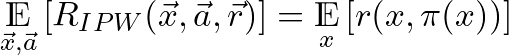
A good policy maximizes the average (expected) reward E[r(x,π(x))]. This expression is the expectation of the reward we get if we use our policy to select the action, averaging across contexts. What makes this challenging is that we observe the reward only for the action we choose for each context. So we only know if our policy is good by trying it out… or can we?
A Counterfactual Performance Estimator
This is actually exactly what counterfactual evaluation methods try to do: estimate how well a policy would have worked if we had used it instead of some “logging policy”. In other words, we’ve recorded the results from our random assignments, how well does a given partitioning rule work?
We’re lucky because we randomly assigned actions, which makes analysis easy (but, as we’ll see, the logging policy need not be purely random). We’ll do something simple: take the average performance over cases where what we randomly chose is the same as what our policy would have done. To simplify notation, let’s introduce some shorthand: xᵢ, aᵢ, rᵢ are the context, assigned treatment, and observed reward for the ith observation, pₐ is the probability of the logging policy taking action a, and N is the total number of observations. The estimator

is unbiased, meaning
This says that the expectation of the estimator taken over draws of datasets is the expected reward using our policy π. In other words, on average, it will be the right estimate! And due to concentration bounds, with large enough data sets it’s likely that any given estimate will be accurate.
Notice that actually nowhere did we use the fact that there is a proper A/B test going on. Rather, all we needed to know is the probability of a logging policy choosing each option, and that those probabilities needed to be >0 for each option, although we’d need to compute a weighted average instead of a simple average if the probabilities weren’t all equal. This is called the “inverse propensity weighting” estimator and is used extensively in Causal, Counterfactual, and Uplift ML literature, as well as econometrics!
Why Divide by pₐᵢ?
In our case where we chose actions randomly as the logging policy, there’s a 50–50 chance that we can “use” a given data point, because there’s a 50–50 chance that our new policy’s decision will line up with one the logging policy used. So otherwise, our estimate would be underestimated by a factor of two.
What if you didn’t run an A/B test? In that case, you need to correct for the fact that the logging policy made decisions your policy wouldn’t have (or at least so frequently). Suppose 9 times out of 10 the logging policy decided to do something bad, resulting in a low reward. If you didn’t divide by the logging probability 9/10 for those data points, you would be scoring your new policy with a lot more of those bad decisions than you should be!
Now, we can take any arbitrary policy and evaluate how good it would have been, using a single dataset recorded up front. This means that not only can we rate how good a policy is, but we can also optimize the policy for counterfactual performance — just like optimizing a normal ML model to minimize, say, the expected squared error.
Since our data was gathered from an A/B test, our problem technically is called Uplift Modeling, which is a subset of Batch Learning from Bandit Feedback (where action probabilities are not all equal, but you’ve logged them), which is a subset of Causal Machine Learning (where you may or may not have a stochastic policy or logs of action probabilities).
Methods for Uplift Modeling
Meta learners
There are many approaches to learn a policy that optimizes for this metric — some directly, some more indirectly. Your first idea might be to forget about what I just said about optimizing the counterfactual risk and instead use your machine learning toolbelt. You’ll just train a classifier to predict which profiles will click if given an email, and which profiles will click if given an SMS. To figure out what you should do for a profile, you’ll see which model has higher predicted probability.
These are actually well-studied methods for Uplift Modeling, falling under the umbrella term of “meta estimators” of individual treatment effects (ITEs). If two separate models are trained, it’s called a “t” estimator. If one model is trained with the treatment encoded as another feature, it’s called an “s” estimator.
These methods are great because they’re simple, generally fast to run, and you automatically get outcome predictions — models of whether someone will engage with an SMS or an Email campaign in this case. But, the fact that in these methods you aren’t directly learning ITEs (the delta between performance an individual has if given one treatment minus performance if given the other) means there are downsides, and they won’t always work as well as you’d like.
There is a class of more complex models, again using out-of-the-box machine learning algorithms, called “r-estimators”. It’s also confusingly referred to as “double ML”, “de-biased ML”, or “orthogonal ML”. They’re a bit too complicated to touch on in this blog post, but Causal Inference for the Brave and True has an excellent and entertaining chapter on them.
Decision Trees
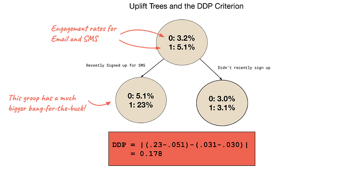
The beauty of decision trees is that all we need is a splitting criterion that describes how “good” the resulting subgroups are. Instead of that criterion being the decrease in the error of the y-variable, as we often use in supervised learning, we can use our counterfactual performance estimator we introduced above, resulting in the CTS criterion. In a similar vein, you could try to maximize the difference in the treatment effect between the subgroups when you split. That results in the DDP criterion, which is shown in the figure below. Or, you could try information theoretic measures, statistical measures, or just building on a simple criterion but with added regularization — the possibilities are endless! Trees can also be ensembled into forests to improve stability.
Importantly, these trees learn ITEs directly, and regularization methods like restricting tree depth appropriately restrict the complexity of the ITEs learned, rather than a proxy.
More ways to learn
As you might expect, work has also gone into directly optimizing the policy by parameterizing it (e.g. with a neural network) and optimizing it with stochastic gradient descent.
Additionally, “doubly robust” learners essentially blend this with the T/S learners. They’re called doubly-robust because they are provably consistent if either learning T/S learners OR the IPW estimate is consistent.
In practice, we found that uplift decision trees using random forest bagging tends to most reliably produce positive results. Other algorithms could produce phenomenal results, but could also produce very incorrect predictions.
Part 3: Automation of Uplift Modeling — Personalization tests
We recently released Personalization Tests, a feature that automates this whole process for Klaviyo customers. Personalization tests, like “pick-a-winner” tests, first run an A/B test on a portion of a campaign’s recipients. We build an uplift model on the A/B test results and then send the remainder of recipients the variation predicted to be best for them. This means that customers who know there’s no “one size fits all” solution when it comes to their messages can click one button to send the right content to each recipient. The diagram below shows what a fitted personalization test model might look like.
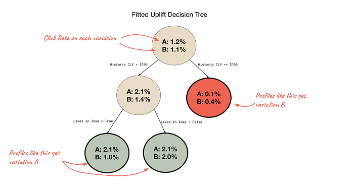
We also explain the learned uplift model to give customers insights into what segments of their customers have different tastes than their other customers and who have higher affinity with which content.

Personalization Tests in Klaviyo
This is just one use case of uplift modeling — we plan to use it across all kinds of features and even to understand our own A/B tests better. It’s a quickly developing field, propelled by clinical trial researchers who want to understand for whom their treatments work and for whom they don’t.
Conclusion
If you want to get started with Uplift Modeling, there are several Python packages like DoWhy, CausalML, and EconML that have implementations of uplift algorithms, Causal Inference methods, and policy optimization. If you want to read more, Causal Inference for the Brave and True by Matheus Facure Alves has some great content on inverse propensity weighting, doubly robust estimation, and meta estimators including Double ML. Susan Athey and Stefan Wager have both published seminal papers in this area, which are worth checking out! Finally, I was privileged to participate in Thorsten Joachims’ seminar on Counterfactual Machine Learning, whose course page is open to the public and has links to lectures and foundational papers.
If you’re interested in working on these kinds of fascinating problems at Klaviyo, visit our career page for opportunities!
Appendix: Proving the IPW estimator is unbiased
Earlier, we imagined the scenario where some users interacting with a “logging” policy (to include random assignment) generated a dataset: there are N observations. For the ith observation, xᵢ, aᵢ, rᵢ are the context, assigned treatment, and observed reward respectively. Let pₐ>0 be the probability of the logging policy taking action a.
To show that the IPW estimator is unbiased, we’ll use the law of total expectation and the definition of an expectation:

Line (1) to (2) pushes in the expectation over actions (recall that we assigned treatments randomly, so these actions are random variables) using the law of total expectation. We also recall the definition of rᵢ as a function of rᵢ and aᵢ. Line (2) to (3) rewrites the expectation using the definition of the expectation. We’re also using the fact that in our case treatments are assigned randomly. Line (3) to (4) just simplifies by canceling out the probabilities. Line (4) to (5) uses the fact that sample averages are unbiased estimators of a mean